tidymodels vs mlr3
Comparison of packages for prediction: {tidymodels} vs. {mlr3}
So I wrote a lot of prediction code for my dissertation using {caret} and I wasn’t interested in learning other frameworks… just because I haven’t had the need to do so. But I’ve learned so much from dabbling around with the {caret} package and I think people that are interested in doing prediction related work will benefit from trying out different packages so I’m writing this post for those interested in looking at what the whole process looks like when using {tidymodels} or {mlr3}. I’m referencing Konrad Semsch since that’s where I got the inspiration to write this post.
A little note about {caret}
I just want to say a quick word about {caret}. If someone is interested in starting out with a book that they can follow along, I would highly recommendt the applied predictive modeling book by Max Kuhn and Kjell Johnson. I started out my journey using {caret} and learned the concept using the book. It’s well written and is a great introduction to machine learning. After going through the book, I think moving on to {tidymodels} or {mlr3} would be super easy. {caret} is a beast in terms of setting up the code to get to doing predictions and other frameworks that have developed afterwards may benefit practitioners given the clarity one may gain through the coding framework. Now let’s dive into how we would do some predictions!
Prediction problem: Predicting ‘Good’ and ‘Bad’ Loans
We’re going to use the credit_data from the {recipes} package.
library('pacman')
p_load(tidymodels, mlr3, recipes, ranger, igraph)

data('credit_data')

credit_data %>% str
## 'data.frame': 4454 obs. of 14 variables:
## $ Status : Factor w/ 2 levels "bad","good": 2 2 1 2 2 2 2 2 2 1 ...
## $ Seniority: int 9 17 10 0 0 1 29 9 0 0 ...
## $ Home : Factor w/ 6 levels "ignore","other",..: 6 6 3 6 6 3 3 4 3 4 ...
## $ Time : int 60 60 36 60 36 60 60 12 60 48 ...
## $ Age : int 30 58 46 24 26 36 44 27 32 41 ...
## $ Marital : Factor w/ 5 levels "divorced","married",..: 2 5 2 4 4 2 2 4 2 2 ...
## $ Records : Factor w/ 2 levels "no","yes": 1 1 2 1 1 1 1 1 1 1 ...
## $ Job : Factor w/ 4 levels "fixed","freelance",..: 2 1 2 1 1 1 1 1 2 4 ...
## $ Expenses : int 73 48 90 63 46 75 75 35 90 90 ...
## $ Income : int 129 131 200 182 107 214 125 80 107 80 ...
## $ Assets : int 0 0 3000 2500 0 3500 10000 0 15000 0 ...
## $ Debt : int 0 0 0 0 0 0 0 0 0 0 ...
## $ Amount : int 800 1000 2000 900 310 650 1600 200 1200 1200 ...
## $ Price : int 846 1658 2985 1325 910 1645 1800 1093 1957 1468 ...Just to be clear, we’re not going to focus too much on some of the aspects of machine learning such as:
- Understanding missingness in the data
- Understanding what the distribution of variables look like and trying to understand all the intricate relationships. We’re going to assume the random forest algorithm will prune those that aren’t important and keep those that are
- Issues of class imbalance.
I’m also going to assume that most who are reading this post have coded at least parts of a machine learning pipeline before.
{tidymodels} framework
Using the the {tidymodels} framework, let’s split the data into training and testing.
split <- initial_split(credit_data, prop = 0.80, strata = "Status")

df_train <- training(split)
df_test  <- testing(split)
Let’s do a 4-fold cross validation to tune the hyperparameters of random forest.
# setup 4 fold cross validation for the training
train_cv <- vfold_cv(df_train, v = 4, strata = "Status")
Next we need to setup a recipe for preprocessing as well as modeling. This entails taking the training data and giving it a formula for random forest, assigning NAs to a new level (‘unknwon’ so the prediction process doesn’t produce errors), median imputation, combining infrequent categories, and creating ‘unrecorded_observation’ level in the training and test set. The last preprocessing is important because many times the cross-validation process will be given a sample where not all levels of a categorical feature/variable is present. In those cases the prediction process will result in an error given the unknown predictor showing up in a test set. The last step step_novel() provides a way to mitigate that.
recipe <- df_train %>%
  # Model formula: Want to predict Status based on all variables in the dataset
  recipe(Status ~ .) %>%

  # Imputation: assigning NAs to a new level for categorical and median imputation for numeric
  step_unknown(all_nominal(), -Status) %>%
  step_impute_median(all_numeric()) %>%

  # Combining infrequent categorical levels and introducing a new level for prediction time
  step_other(all_nominal(), -Status, other = "infrequent_combined") %>%
  step_novel(all_nominal(), -Status, new_level = "unrecorded_observation") %>%

  # Hot-encoding categorical variables
  step_dummy(all_nominal(), -Status, one_hot = TRUE)
Now we’ll specify the random forest algorithm to be used.
# Specify model engine
(engine_tidym <- rand_forest(
  mode = "classification",
  mtry = tune(),
  trees = tune(),
  min_n = tune()
) %>%
    set_engine("ranger", importance = "impurity")) # you can provide additional, engine specific arguments to '...'
## Random Forest Model Specification (classification)
##
## Main Arguments:
## mtry = tune()
## trees = tune()
## min_n = tune()
##
## Engine-Specific Arguments:
## importance = impurity
##
## Computational engine: rangerNext we need to specify the search space (grid) of hyperparameter values to find the optimal set of hyperparameters to be used for the final prediction process.
# Specifying the grid of hyperparameters that should be tested
(gridy_tidym <- grid_random(
  mtry() %>% range_set(c(1, 20)),
  trees() %>% range_set(c(500, 1000)),
  min_n() %>% range_set(c(2, 10)),
  size = 5
))
## # A tibble: 5 x 3
## mtry trees min_n
## <int> <int> <int>
## 1 9 544 3
## 2 5 933 7
## 3 18 853 10
## 4 8 747 4
## 5 18 526 5Lastly, we’ll set the whole predictino process as a workflow.
# COmbine modeling recipe into a worklow
wkfl_tidym <- workflow() %>%
  add_recipe(recipe) %>%
  add_model(engine_tidym)
Next we are going to actually tune the model to find the optimal hyperparameters. We want to optimize this process by using {doParallel} to speed up the resampling process.
# Find best hyperparameters
# load parallel package
# Looks like the doFuture hasn't implemented a RNG seed that will allow reproducible parallel resampling
p_load(doParallel)
cl <- makeCluster(parallel::detectCores())
registerDoParallel(cl)

grid_tidym <- tune_grid(
  wkfl_tidym,
  resamples = train_cv,
  grid = gridy_tidym,
  # Use Area under the roc curve
  metrics = metric_set(roc_auc),
  # Save predictions
  # Parallel processing link:https://www.tmwr.org/grid-search.html
  control = control_grid(allow_par = TRUE, save_pred = TRUE, parallel_over = 'resamples')
  # Non parallel version
  # control = control_grid(save_pred = TRUE)
)
Let’s now take a look at the 4-fold cross validation results
print(grid_tidym)## # Tuning results
## # 4-fold cross-validation using stratification
## # A tibble: 4 x 5
## splits id .metrics .notes .predictions
## <list> <chr> <list> <list> <list>
## 1 <split [2673/8… Fold1 <tibble[,7] [5 ×… <tibble[,1] [0 ×… <tibble[,8] [4,460 …
## 2 <split [2674/8… Fold2 <tibble[,7] [5 ×… <tibble[,1] [0 ×… <tibble[,8] [4,455 …
## 3 <split [2674/8… Fold3 <tibble[,7] [5 ×… <tibble[,1] [0 ×… <tibble[,8] [4,455 …
## 4 <split [2674/8… Fold4 <tibble[,7] [5 ×… <tibble[,1] [0 ×… <tibble[,8] [4,455 …Aggregate the performance metrics for each hypermarater combinations across all cv folds to find best performing hyperparameter set to use in the final model.
collect_metrics(grid_tidym)## # A tibble: 5 x 9
## mtry trees min_n .metric .estimator mean n std_err .config
## <int> <int> <int> <chr> <chr> <dbl> <int> <dbl> <chr>
## 1 9 544 3 roc_auc binary 0.830 4 0.0103 Preprocessor1_Model1
## 2 5 933 7 roc_auc binary 0.834 4 0.00930 Preprocessor1_Model2
## 3 18 853 10 roc_auc binary 0.830 4 0.0103 Preprocessor1_Model3
## 4 8 747 4 roc_auc binary 0.833 4 0.00988 Preprocessor1_Model4
## 5 18 526 5 roc_auc binary 0.828 4 0.0105 Preprocessor1_Model5We’re going to select the best set of parameters and run the final prediction on the test set.
grid_tidym_best <- select_best(grid_tidym)
# Propagate the best set of parameters into the final workflow
(wkfl_tidym_best <- finalize_workflow(wkfl_tidym, grid_tidym_best))
## ══ Workflow ════════════════════════════════════════════════════════════════════
## Preprocessor: Recipe
## Model: rand_forest()
##
## ── Preprocessor ────────────────────────────────────────────────────────────────
## 5 Recipe Steps
##
## • step_unknown()
## • step_impute_median()
## • step_other()
## • step_novel()
## • step_dummy()
##
## ── Model ───────────────────────────────────────────────────────────────────────
## Random Forest Model Specification (classification)
##
## Main Arguments:
## mtry = 5
## trees = 933
## min_n = 7
##
## Engine-Specific Arguments:
## importance = impurity
##
## Computational engine: ranger# finally fit the final model using the best parameter set on the split created before
(wkfl_tidym_final <- last_fit(wkfl_tidym_best, split = split))## # Resampling results
## # Manual resampling
## # A tibble: 1 x 6
## splits id .metrics .notes .predictions .workflow
## <list> <chr> <list> <list> <list> <list>
## 1 <split [356… train/tes… <tibble[,4] [… <tibble[,1]… <tibble[,6] [88… <workflo…We can now check the performance of the model using the sets of hyperparameters on the training set
percent(show_best(grid_tidym, n = 1)$mean)## [1] "83%"Likelye, let’s check the performance of the model using the best set of hyperparameters on the test set
percent(wkfl_tidym_final$.metrics[[1]]$.estimate[[2]])## [1] "81%"Lastly, we’re going to take a look at the variable importance.
p_load(vip)
vip(pull_workflow_fit(wkfl_tidym_final$.workflow[[1]]))$data
## # A tibble: 10 x 2
## Variable Importance
## <chr> <dbl>
## 1 Income 134.
## 2 Seniority 131.
## 3 Amount 113.
## 4 Price 105.
## 5 Age 86.1
## 6 Assets 81.0
## 7 Expenses 61.4
## 8 Records_yes 54.9
## 9 Records_no 54.1
## 10 Time 43.4We can stop the clusters specified before now. Remember not to stopCluster too early because this may screw up the prediction process on the test set. Not sure what is happening but will need to investigate to further understand the test set prediction mechanism.
stopCluster(cl){mlr3} framework
With {mlr3}, I personally think the preprocessing step doesn’t have a lot of functionality as the {tidymodels} framework but the nested resampling procedure looks more straightforward and clean. Let’s load the packages and go through some of the steps in {mlr3} now.
p_load(mlr3, mlr3learners)

# create learning task
task_credit <- TaskClassif$new(id = "credit", backend = credit_data, target = "Status")
task_credit
## <TaskClassif:credit> (4454 x 14)
## * Target: Status
## * Properties: twoclass
## * Features (13):
## - int (9): Age, Amount, Assets, Debt, Expenses, Income, Price,
## Seniority, Time
## - fct (4): Home, Job, Marital, RecordsWe don’t necessarily need to split the data like we did for {tidymodels}. Let’s also load the random forest learner that we’ll use for the cross validation for tuning the hyperparameters. We need to also specify the resampling strategy (4 fold cross validation) and the metric we’ll use (AUROC) for assessing the performance of the models.
# load learner
learner <- lrn("classif.ranger", predict_type = "prob")

# specify the resampling strategy... we'll use 4-fold cross-validation
cv_4 = rsmp("cv",folds=4)
measure = msr("classif.auc")
Now we need to setup the tuning process. Let’s first setup the tuning termination object. We set trm('evals',n_evals=20) such that for every resampling fold we’ll stop at 20 random grid searched sets of parameters.
# We also need to specify if we're going to trim the tuning process.. we won't
p_load(mlr3tuning)
eval20 <- trm('evals',n_evals=5)
# for no termination restriction
# evalnon <- trm('none')
We also want to setup the preprocessing similar to how we did it using the {tidymodels} framework. This involves a pipline approach by setting up pipline operations po(). One difference between the ’{tidymodels}framework on the{mlr3}framework is that thestep_unknown(),step_other()andstep_novel()does not seem to exist for the{mlr3}` framework.
# We're also going to utilize the {mlr3pipelines} package framework. We need to basically string together the preprcoessing, hyper parameter tuning, and final
p_load(mlr3pipelines)

# I have not found a easy way to convert NA values to  'unknown' so we'll just go ahead and impute the class labels for the factor variables
sampleimpute <- po('imputesample')

# The below code should work but doesn't for some reason
# mutate$param_set$values$mutation <- list(
#   # across(where(is.factor), ~ifelse(is.na(.),"unknown",.))
#   Home = ~ ifelse(is.na(Home), "unknown",Home),
#   Job = ~ ifelse(is.na(Job), "unknown",Job),
#   Marital = ~ ifelse(is.na(Marital), "unknown",Marital)
# )

# median imputation for missing numeric
medimpute <- po("imputemedian")

# The combining of infrequent categories not an easy task in mlr3 framework
# ALso step_novel like function does not exist in mlr3

# Lastly one-hot encoding
ohencode <- po("encode")

graph <- sampleimpute %>>%
# graph <- mutate %>>%
  medimpute %>>%
  ohencode %>>%
  learner
Another framework the {mlr3} ecosystem utilize is a GraphLearner which takes graphs and strings together the preprocessing, hyperparameter tuning, and prediction process as a Graph Network. I won’t go into the details but if you’re interested you should check out this page.
# Generate graph learner to combine preprocessing, tuning, and predicting
glrn = GraphLearner$new(graph)

# Tuning the same 3 parameters mtry  trees min_n

# Previously with tidymodels we used the below:
# mtry() %>% range_set(c(1, 20)),
# trees() %>% range_set(c(500, 1000)),
# min_n() %>% range_set(c(2, 10)),

# Notice the name of the parameters is different from what was used in the `{tidymodels}` framework.
p_load(paradox)
search_space = ps(
  classif.ranger.mtry = p_int(lower = 1, upper = 10),
  classif.ranger.num.trees = p_int(lower = 500, upper = 1000),
  classif.ranger.min.node.size = p_int(lower = 2, upper = 10)
)
We can also take a look at the whole machine learning pipeline through the graph plot.
# Check graph of the whole process
graph$plot(html=FALSE)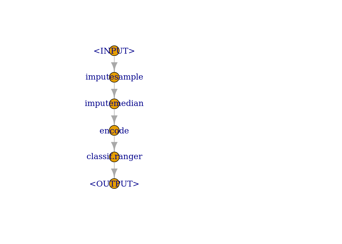
Now let’s generate a AutoTuner class object such that we can run the inner resampling for hyperparater tuning with it. We’re going to do a random grid search on the hyperparameter space based on the search_space constructed and terminate after 20 evaulations. I also have code commented out below that one can use if they want to do a grid search with \(5^\text{(N of hyperparameters)}\).
# Nested resampling for parameter tuning as well as prediction
# This whole nested resampling could be expensive so use multiprocess
at = AutoTuner$new(
  glrn,
  cv_4,
  measure,
  eval20,
  tnr("random_search"),
  search_space,
  store_tuning_instance = TRUE
  )

# for random grid search with 20 combination searched use below
# tuner = tnr("random_search")
# for grid search with specific resolution (i.e. 5 means 5^n parameters)
# tuner = tnr("grid_search", resolution=5)
For the outer resampling (i.e., test set evaluation), we’ll do a holdout resampling to test the best hyperparameter set from the training data on 20% of the test set data.
# We will use a holdout resample for the outer split so that we have 20% as a test set
resampling_outer <- rsmp('holdout', ratio = 0.8)
# resampling_outer <- rsmp('cv', folds = 3)
Since we want to run this whole thing in a parallel fashion, we’ll use the {future} package.
future::plan('multisession')Now we’re ready to run the nested resampling task. We’re going to store the models in order to evaluate the performance of the inner resampling (use store_models=TRUE)
rr <- resample(
  task = task_credit, learner = at, resampling = resampling_outer, store_models = TRUE
  )
## INFO [11:07:18.254] [mlr3] Applying learner 'imputesample.imputemedian.encode.classif.ranger.tuned' on task 'credit' (iter 1/1)
## INFO [11:07:18.592] [bbotk] Starting to optimize 3 parameter(s) with '<OptimizerRandomSearch>' and '<TerminatorEvals> [n_evals=5]'
## INFO [11:07:18.650] [bbotk] Evaluating 1 configuration(s)
## INFO [11:07:18.703] [mlr3] Running benchmark with 4 resampling iterations
## INFO [11:07:18.725] [mlr3] Applying learner 'imputesample.imputemedian.encode.classif.ranger' on task 'credit' (iter 3/4)
## INFO [11:07:21.275] [mlr3] Applying learner 'imputesample.imputemedian.encode.classif.ranger' on task 'credit' (iter 2/4)
## INFO [11:07:22.895] [mlr3] Applying learner 'imputesample.imputemedian.encode.classif.ranger' on task 'credit' (iter 4/4)
## INFO [11:07:24.569] [mlr3] Applying learner 'imputesample.imputemedian.encode.classif.ranger' on task 'credit' (iter 1/4)
## INFO [11:07:26.293] [mlr3] Finished benchmark
## INFO [11:07:26.365] [bbotk] Result of batch 1:
## INFO [11:07:26.369] [bbotk] classif.ranger.mtry classif.ranger.num.trees classif.ranger.min.node.size
## INFO [11:07:26.369] [bbotk] 3 713 9
## INFO [11:07:26.369] [bbotk] classif.auc uhash
## INFO [11:07:26.369] [bbotk] 0.8327978 1fd24ee7-55a6-49a4-ac21-301d37d054e9
## INFO [11:07:26.375] [bbotk] Evaluating 1 configuration(s)
## INFO [11:07:26.425] [mlr3] Running benchmark with 4 resampling iterations
## INFO [11:07:26.434] [mlr3] Applying learner 'imputesample.imputemedian.encode.classif.ranger' on task 'credit' (iter 1/4)
## INFO [11:07:29.606] [mlr3] Applying learner 'imputesample.imputemedian.encode.classif.ranger' on task 'credit' (iter 3/4)
## INFO [11:07:33.068] [mlr3] Applying learner 'imputesample.imputemedian.encode.classif.ranger' on task 'credit' (iter 4/4)
## INFO [11:07:36.436] [mlr3] Applying learner 'imputesample.imputemedian.encode.classif.ranger' on task 'credit' (iter 2/4)
## INFO [11:07:39.727] [mlr3] Finished benchmark
## INFO [11:07:39.831] [bbotk] Result of batch 2:
## INFO [11:07:39.833] [bbotk] classif.ranger.mtry classif.ranger.num.trees classif.ranger.min.node.size
## INFO [11:07:39.833] [bbotk] 6 981 2
## INFO [11:07:39.833] [bbotk] classif.auc uhash
## INFO [11:07:39.833] [bbotk] 0.8291453 0ed1c7fe-605f-4e81-89b9-7cb55366f9a4
## INFO [11:07:39.838] [bbotk] Evaluating 1 configuration(s)
## INFO [11:07:39.878] [mlr3] Running benchmark with 4 resampling iterations
## INFO [11:07:39.885] [mlr3] Applying learner 'imputesample.imputemedian.encode.classif.ranger' on task 'credit' (iter 4/4)
## INFO [11:07:40.806] [mlr3] Applying learner 'imputesample.imputemedian.encode.classif.ranger' on task 'credit' (iter 3/4)
## INFO [11:07:41.687] [mlr3] Applying learner 'imputesample.imputemedian.encode.classif.ranger' on task 'credit' (iter 1/4)
## INFO [11:07:42.568] [mlr3] Applying learner 'imputesample.imputemedian.encode.classif.ranger' on task 'credit' (iter 2/4)
## INFO [11:07:43.506] [mlr3] Finished benchmark
## INFO [11:07:43.573] [bbotk] Result of batch 3:
## INFO [11:07:43.575] [bbotk] classif.ranger.mtry classif.ranger.num.trees classif.ranger.min.node.size
## INFO [11:07:43.575] [bbotk] 1 882 5
## INFO [11:07:43.575] [bbotk] classif.auc uhash
## INFO [11:07:43.575] [bbotk] 0.8237262 537e29c1-b965-49c3-9c20-b3a41a9dd07e
## INFO [11:07:43.580] [bbotk] Evaluating 1 configuration(s)
## INFO [11:07:43.621] [mlr3] Running benchmark with 4 resampling iterations
## INFO [11:07:43.628] [mlr3] Applying learner 'imputesample.imputemedian.encode.classif.ranger' on task 'credit' (iter 1/4)
## INFO [11:07:45.782] [mlr3] Applying learner 'imputesample.imputemedian.encode.classif.ranger' on task 'credit' (iter 3/4)
## INFO [11:07:47.686] [mlr3] Applying learner 'imputesample.imputemedian.encode.classif.ranger' on task 'credit' (iter 4/4)
## INFO [11:07:49.640] [mlr3] Applying learner 'imputesample.imputemedian.encode.classif.ranger' on task 'credit' (iter 2/4)
## INFO [11:07:51.664] [mlr3] Finished benchmark
## INFO [11:07:51.740] [bbotk] Result of batch 4:
## INFO [11:07:51.742] [bbotk] classif.ranger.mtry classif.ranger.num.trees classif.ranger.min.node.size
## INFO [11:07:51.742] [bbotk] 6 622 7
## INFO [11:07:51.742] [bbotk] classif.auc uhash
## INFO [11:07:51.742] [bbotk] 0.8291652 c0be6817-49fb-4cbd-928a-5dabc538ff8c
## INFO [11:07:51.746] [bbotk] Evaluating 1 configuration(s)
## INFO [11:07:51.785] [mlr3] Running benchmark with 4 resampling iterations
## INFO [11:07:51.792] [mlr3] Applying learner 'imputesample.imputemedian.encode.classif.ranger' on task 'credit' (iter 1/4)
## INFO [11:07:53.668] [mlr3] Applying learner 'imputesample.imputemedian.encode.classif.ranger' on task 'credit' (iter 4/4)
## INFO [11:07:55.543] [mlr3] Applying learner 'imputesample.imputemedian.encode.classif.ranger' on task 'credit' (iter 2/4)
## INFO [11:07:57.432] [mlr3] Applying learner 'imputesample.imputemedian.encode.classif.ranger' on task 'credit' (iter 3/4)
## INFO [11:07:59.394] [mlr3] Finished benchmark
## INFO [11:07:59.468] [bbotk] Result of batch 5:
## INFO [11:07:59.470] [bbotk] classif.ranger.mtry classif.ranger.num.trees classif.ranger.min.node.size
## INFO [11:07:59.470] [bbotk] 8 584 10
## INFO [11:07:59.470] [bbotk] classif.auc uhash
## INFO [11:07:59.470] [bbotk] 0.8298606 eb98c038-eebd-4d4a-8c54-0f4c8086fb77
## INFO [11:07:59.481] [bbotk] Finished optimizing after 5 evaluation(s)
## INFO [11:07:59.482] [bbotk] Result:
## INFO [11:07:59.484] [bbotk] classif.ranger.mtry classif.ranger.num.trees classif.ranger.min.node.size
## INFO [11:07:59.484] [bbotk] 3 713 9
## INFO [11:07:59.484] [bbotk] learner_param_vals x_domain classif.auc
## INFO [11:07:59.484] [bbotk] <list[5]> <list[3]> 0.8327978Let’s check the tuning results.
# The final hyper parameter selected and the training set AUC results
rr$learners[[1]]$tuning_result
## classif.ranger.mtry classif.ranger.num.trees classif.ranger.min.node.size
## 1: 3 713 9
## learner_param_vals x_domain classif.auc
## 1: <list[5]> <list[3]> 0.8327978# Aggregate performance from the 3 outer resampling datasets after the 5 inner resampling for hyperparameter tuningThe test set results are presented below.
# Using the hyper parameter selected from the training set if we predict using the test set we get the below
rr$score(msr("classif.auc"))
## task task_id learner
## 1: <TaskClassif[46]> credit <AutoTuner[38]>
## learner_id
## 1: imputesample.imputemedian.encode.classif.ranger.tuned
## resampling resampling_id iteration prediction
## 1: <ResamplingHoldout[19]> holdout 1 <PredictionClassif[19]>
## classif.auc
## 1: 0.8146165rr$aggregate(msr("classif.auc"))## classif.auc
## 0.8146165rr$prediction()$confusion## truth
## response bad good
## bad 95 53
## good 153 590Let’s visualize the test set predictions now.
# Plots
p_load(mlr3viz,precrec)

autoplot(rr, measure = msr('classif.auc'))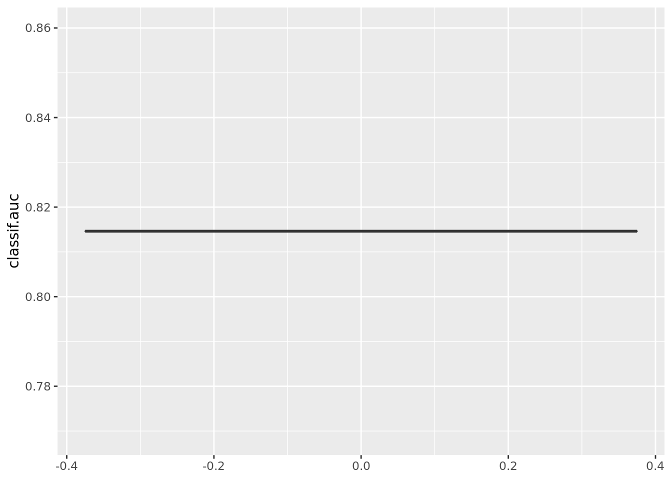
autoplot(rr, type = "histogram")## `stat_bin()` using `bins = 30`. Pick better value with `binwidth`.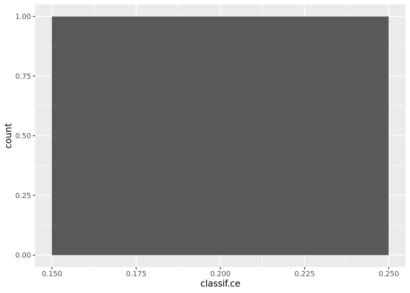
autoplot(rr, type = "roc")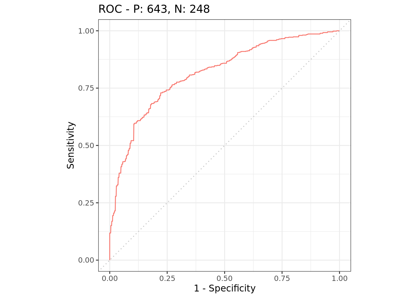
autoplot(rr, type = "prc")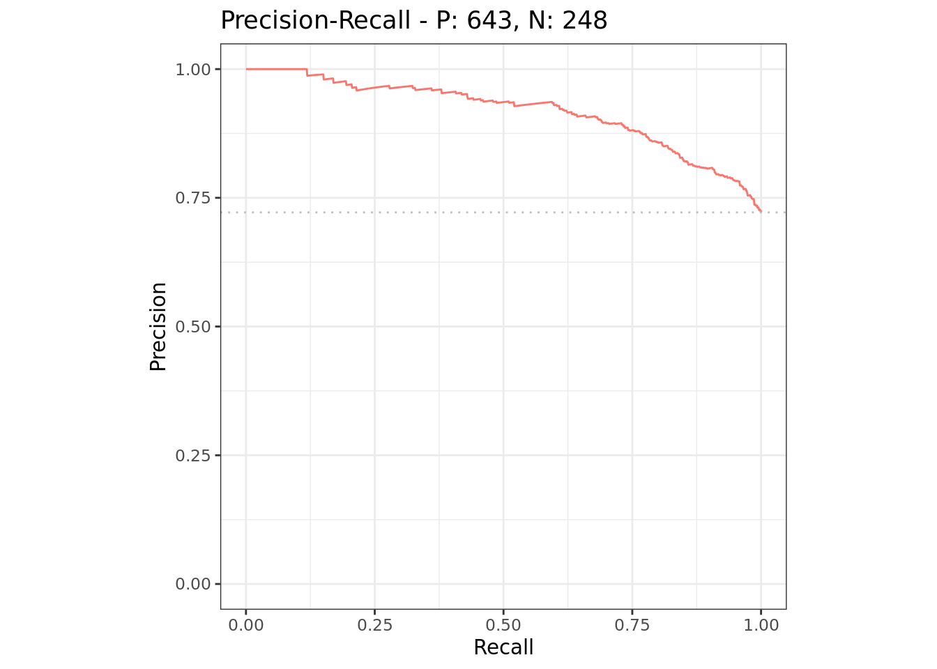
There you have it!
Conclusion
Overall, I like both frameworks but it looks like both have a few areas that could improve. Overall, both development team has done a great job and I’ll likely use both frameworks so that I can benefit from what both packages offer. I hope the above codes were helpful and I’ll likely be posting a few more analyses using both packages so stay tuned!
Chong H. Kim
Health Economics & Outcomes Researcher
My research interests include health economics & outcomes research (HEOR), real-world evidence/observation research, predictive modeling, and spatial statistics.