Sample Size Calculation with R Extended
Sample Size Caluclation in R… Extended!
This is an extension from a post I saw here. When thinking about study designs for a trial that we want to conduct for a client, one of the things that we need to think about is how many patients we would need to recruit to see the effect that we propose to see? We’re going to walk through a couple of scenarios and see how we need can use R to get at the sample size & power question when desgining our studies.
Scenario 1: One Sample Mean T-Test
There aren’t many scenarios where we want to test one population and if they have a significantly differing values of a parameter of interest from a null value. But let’s start with an easy example first.
Let’s say we’re interested determining if the average hospital cost of patients with hemophilia is less than $80,000 a year. We collect trial data. The data is shown below.
df_s1 <- data.frame(
  cost_hosp = c(70000,80000,2000,13000,140000,13000,24000,44000,87000,30000)
)

# load library to summarize data
library('pacman')
p_load(skimr,dplyr)
df_s1 %>%
skim()| Name | Piped data |
| Number of rows | 10 |
| Number of columns | 1 |
| _______________________ | |
| Column type frequency: | |
| numeric | 1 |
| ________________________ | |
| Group variables | None |
Variable type: numeric
| skim_variable | n_missing | complete_rate | mean | sd | p0 | p25 | p50 | p75 | p100 | hist |
|---|---|---|---|---|---|---|---|---|---|---|
| cost_hosp | 0 | 1 | 50300 | 43361.66 | 2000 | 15750 | 37000 | 77500 | 140000 | ▇▃▃▂▂ |
Now that we have a sense of the data, we need to extract the effect size in order to estimate the number of patients we need to survey/collect for our study. The equation for effect size is as below
\[ \text{effect size} = \frac{\text{mean}_{\text{sample}} - \text{mean}_{\text{hypothesized}}}{\text{standard deviation}_{\text{sample}}} \] Below is the R code for calculating the effect size
effsize <- (mean(df_s1$cost_hosp)  - 80000) / sd(df_s1$cost_hosp)
effsize
## [1] -0.6849369Now we can use the {pwr} package to estimate the sample size needed. We’re going to assume an of 0.05 and power of 0.80. The hypothesis of interest is whether the estimated cost from our sample is smaller than $80,000.
p_load(pwr)
pwr.t.test(d = effsize, sig.level =0.05, power=0.80, type = "one.sample", alternative= "less")
##
## One-sample t test power calculation
##
## n = 14.63024
## d = -0.6849369
## sig.level = 0.05
## power = 0.8
## alternative = lessGiven that we see the number going over 14, we need to round up and collect information from 15 patients.
Now let’s say we’re interested in instances where different countries have different mean costs and therefore we’d be interested to see how our sample sizes need to pan out in different countries. See the data below:
df_s1b <- data.frame(
  cost_hosp_usa = c(70000,80000,2000,13000,140000,13000,24000,44000,87000,30000),
  cost_hosp_china = c(20000,24000,2300,15000,40000,6300,9400,10000,27000,23000),
  cost_hosp_korea = c(30000,40000,3000,10000,100000,3500,14000,23000,87000,30000)
)

df_s1b %>%
skim()| Name | Piped data |
| Number of rows | 10 |
| Number of columns | 3 |
| _______________________ | |
| Column type frequency: | |
| numeric | 3 |
| ________________________ | |
| Group variables | None |
Variable type: numeric
| skim_variable | n_missing | complete_rate | mean | sd | p0 | p25 | p50 | p75 | p100 | hist |
|---|---|---|---|---|---|---|---|---|---|---|
| cost_hosp_usa | 0 | 1 | 50300 | 43361.66 | 2000 | 15750 | 37000 | 77500 | 140000 | ▇▃▃▂▂ |
| cost_hosp_china | 0 | 1 | 17700 | 11350.18 | 2300 | 9550 | 17500 | 23750 | 40000 | ▇▅▇▂▂ |
| cost_hosp_korea | 0 | 1 | 34050 | 33700.02 | 3000 | 11000 | 26500 | 37500 | 100000 | ▇▇▁▁▃ |
Let’s create a effect size df now
effsizedf <- data.frame(
  es = c((mean(df_s1b$cost_hosp_usa)  - 80000) / sd(df_s1b$cost_hosp_usa) , (mean(df_s1b$cost_hosp_china)  - 80000) / sd(df_s1b$cost_hosp_china), (mean(df_s1b$cost_hosp_korea)  - 80000) / sd(df_s1b$cost_hosp_korea)),
  country = c("USA","China","Korea")
)
effsizedf
## es country
## 1 -0.6849369 USA
## 2 -5.4888980 China
## 3 -1.3635005 KoreaUsing the effsizedf we’re going to create another data.frame that will give us the estimated sample size to arrive at the effect estimate. We’re going to use{purrr} to apply the pwr.t.test function across the rows of the effsizedf.
p_load(purrr)

ss_s1 <- effsizedf %>%
  pmap_dfr(function(es, country){
    data.frame(
      country = country,
      es = es,
      n = ceiling(pwr.t.test(d = es, sig.level =0.05, power=0.80, type = "one.sample", alternative= "less")$n)
    )
  })
ss_s1
## country es n
## 1 USA -0.6849369 15
## 2 China -5.4888980 3
## 3 Korea -1.3635005 5To make it easier on the eyes let’s visualize it using {ggplot2}.
p_load(ggplot2)

p<-ggplot(data=ss_s1, aes(x=country, y=n, fill=country, label=n)) +
  geom_bar(stat="identity") +
  geom_text(nudge_y = 1) +
  theme_light() +
  theme(legend.position = "none") +
  xlab("") + ylab("Number of Patients Needed")
p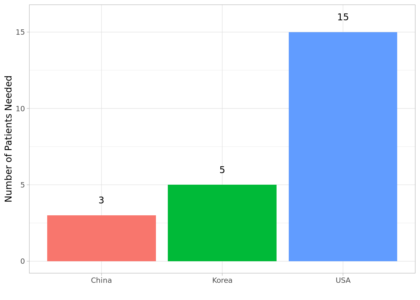
So there you have it. As the importance of real-world evidence is continuing to grow and emphasis on generating value continues to rise, I hope more people will be able to utilize codes written in R (or python or SAS) when designing real-world studies.
I’ll be editing this post from time to time to add more power & sample size calculations for different tests. Thank you for reading and happy coding!
Chong H. Kim
Health Economics & Outcomes Researcher
My research interests include health economics & outcomes research (HEOR), real-world evidence/observation research, predictive modeling, and spatial statistics.