Matching with {MatchIt}

Many observational studies that are published try to balance the demographic and clinical characteristics that may be associated with the primary exposure of interest (e.g., drug or intervention) and the outcome of interest (e.g., time to relapse). Of the matching approaches, I’m going to cover the code for propensity score matching (PSM) and direct matching.

I’ve had many projects where PSM was done in order to balance the potential confounding characteristics between two cohorts. For example, a cohort that was prescribed drug A and a cohort that was prescribed drug B. This is important because this allows the effect of the drugs to be quantified and be characterized while minimizing the potential confounding effect of other characteristics such as age, gender, and comorbidities.

We’re going to use the Mayo Clinic Primary Biliary Cholangitis Data and only use patients that were censored and died.

Data setup

library('pacman')
p_load(survival,dplyr,MatchIt)
data("pbc")

pbc_final <- pbc %>%
  filter(status %in% c(0,2)) %>%
  filter(!is.na(trt)) %>%
  mutate(trt = ifelse(trt == 1, 1, 0))

Propensity Score Matching

First we need to generate the propensity scores for patients that were treated vs non-treated. Many folks use a logistic regression model to generate the p-values based on regressing the confounding variables on the treatment variable. Lastly, a 0.1 SD caliper is used.

Note: missing values are not allowed in the treatment.

m.out <- matchit(trt ~ age + sex + stage, 
                 data = pbc_final, method = "nearest", caliper = 0.1)

## Warning: Fewer control units than treated units; not all treated units will get
## a match.

Sometimes, there aren’t enough control units compared to the treated units therefore not all treated units will get a match

summary(m.out)

## 
## Call:
## matchit(formula = trt ~ age + sex + stage, data = pbc_final, 
##     method = "nearest", caliper = 0.1)
## 
## Summary of Balance for All Data:
##          Means Treated Means Control Std. Mean Diff. Var. Ratio eCDF Mean
## distance        0.5213        0.4886          0.3510     1.2020    0.0996
## age            52.1431       49.0098          0.2882     1.1745    0.0863
## sexm            0.1216        0.1034          0.0556          .    0.0182
## sexf            0.8784        0.8966         -0.0556          .    0.0182
## stage           2.9527        3.0828         -0.1369     1.3679    0.0325
##          eCDF Max
## distance   0.1909
## age        0.1556
## sexm       0.0182
## sexf       0.0182
## stage      0.0763
## 
## 
## Summary of Balance for Matched Data:
##          Means Treated Means Control Std. Mean Diff. Var. Ratio eCDF Mean
## distance        0.5045        0.5009          0.0383     1.0152    0.0136
## age            50.4136       50.0052          0.0376     0.9795    0.0253
## sexm            0.1261        0.1092          0.0514          .    0.0168
## sexf            0.8739        0.8908         -0.0514          .    0.0168
## stage           3.0000        3.0084         -0.0088     1.2841    0.0273
##          eCDF Max Std. Pair Dist.
## distance   0.0504          0.0439
## age        0.0756          0.6067
## sexm       0.0168          0.6685
## sexf       0.0168          0.6685
## stage      0.0588          0.9111
## 
## Percent Balance Improvement:
##          Std. Mean Diff. Var. Ratio eCDF Mean eCDF Max
## distance            89.1       91.8      86.3     73.6
## age                 87.0       87.1      70.7     51.4
## sexm                 7.5          .       7.5      7.5
## sexf                 7.5          .       7.5      7.5
## stage               93.5       20.2      16.0     22.9
## 
## Sample Sizes:
##           Control Treated
## All           145     148
## Matched       119     119
## Unmatched      26      29
## Discarded       0       0

With the summary statement, we can get access to the matched sample as well as understand the number of patients that weren’t matched.

We can also generate a plot to see what the covariate balance looks like

plot(summary(m.out))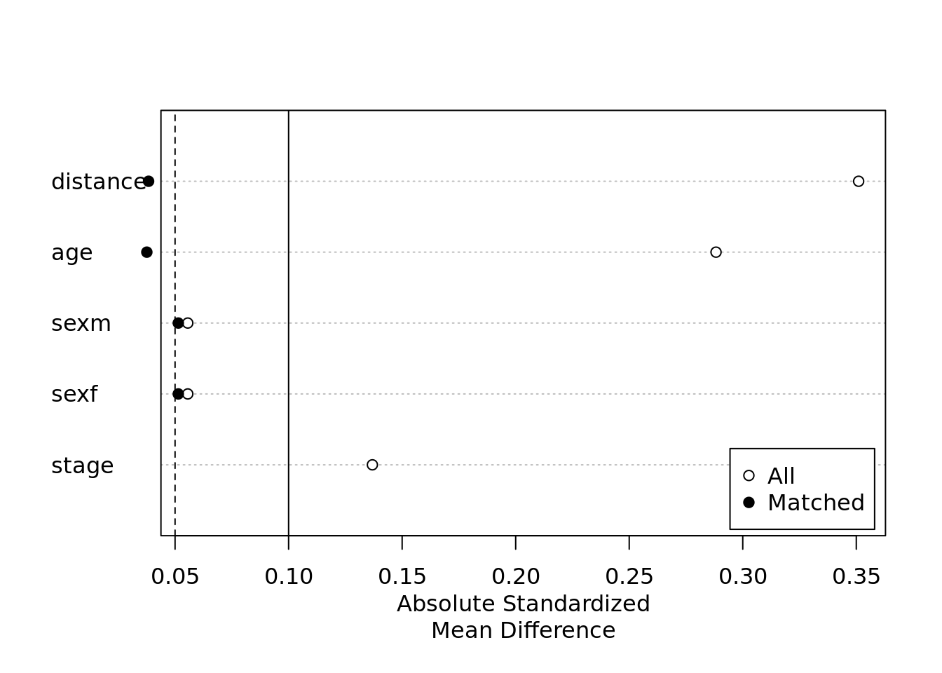

You can see that the Absolute Standardized Mean Difference is now very close to 0 for almost all of the variables which is what you want when matching the patients according to their characteristics.

Now let’s take a look at direct matching

Direct matching

Where PSM matches patients based on the propensity score, a direct matching approach is based on finding an exact match from one group to another. For example a patient prescribed drug A who is 55 years old and a female should be matched to a patient prescribed drug B who is 55 years old and a female as well.

Let’s take a look at the code

m.out.exact <- matchit(trt ~ age + sex + status, 
                 data = pbc_final, method = "nearest", 
                 exact = c("age","sex","status"), ratio = 1)

## Warning: Fewer control units than treated units in some 'exact' strata; not all
## treated units will get a match.

Notice that the method is still “nearest” but we provide a exact = c("age","sex","status") argument which specifies to the function that we want to match patients exactly on age, sex, and status. Let’s take a look at the summary of the matching process.

summary(m.out.exact)

## 
## Call:
## matchit(formula = trt ~ age + sex + status, data = pbc_final, 
##     method = "nearest", exact = c("age", "sex", "status"), ratio = 1)
## 
## Summary of Balance for All Data:
##          Means Treated Means Control Std. Mean Diff. Var. Ratio eCDF Mean
## distance        0.5161        0.4939          0.2882     1.1800    0.0855
## age            52.1431       49.0098          0.2882     1.1745    0.0863
## sexm            0.1216        0.1034          0.0556          .    0.0182
## sexf            0.8784        0.8966         -0.0556          .    0.0182
## status          0.8784        0.8276          0.0510     1.0152    0.0127
##          eCDF Max
## distance   0.1521
## age        0.1556
## sexm       0.0182
## sexf       0.0182
## status     0.0254
## 
## 
## Summary of Balance for Matched Data:
##          Means Treated Means Control Std. Mean Diff. Var. Ratio eCDF Mean
## distance        0.5467        0.5467               0          1         0
## age            55.8535       55.8535               0          1         0
## sexm            0.0000        0.0000               0          .         0
## sexf            1.0000        1.0000               0          .         0
## status          0.0000        0.0000               0          .         0
##          eCDF Max Std. Pair Dist.
## distance        0               0
## age             0               0
## sexm            0               0
## sexf            0               0
## status          0               0
## 
## Percent Balance Improvement:
##          Std. Mean Diff. Var. Ratio eCDF Mean eCDF Max
## distance             100        100       100      100
## age                  100        100       100      100
## sexm                 100          .       100      100
## sexf                 100          .       100      100
## status               100          .       100      100
## 
## Sample Sizes:
##           Control Treated
## All           145     148
## Matched         2       2
## Unmatched     143     146
## Discarded       0       0

We were only able to match 2 patients…. This isn’t great because we would want to include more patients in our analysis and be able to show the effect of drug A and drug B on the outcomes.

plot(summary(m.out.exact))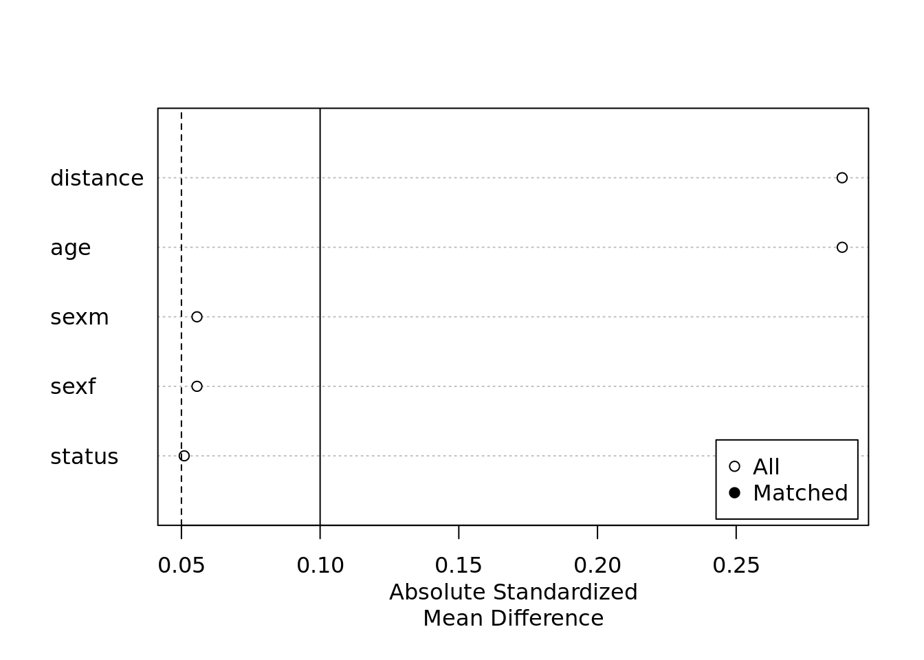

In theory you would want a large enough sample before matching so when you do indeed do the matching, you might lose a substantial amount but should be able to carry out the modeling such that the estimates of interest are obtainable.

I hope this was helpful. Assessing the impact of interventions via an analysis that hopes to contain potential confounding effect can be somewhat of a mental challenge during the design phase. The code above is actually the easy part but the hard part is figuring out what variables should be included in the matching process and what other matching procedures should be explored before settling on a final matching approach. I hope this will be useful for someone embarking upon a PSM or direct matching procedure for their observational analysis! Good luck to everyone who needs to do so!